Physical modeling and machine learning in oscillating heat pipes
1. Oscillating heat pipes
Thermal management has become one of the major bottlenecks in the development of new-generation technologies, ranging from the miniaturization of computer processors to hypersonic vehicles. Oscillating heat pipes (OHPs) have the potential to address some of these pressing thermal needs due to their staggering thermal conductivity, absence of mechanical parts, and simplicity of design. An OHP is a special kind of heat pipe that consists of a meandering capillary partially filled with a working fluid (Ma, 2015). A typical OHP consists of an evaporator and a condenser joined by an intermediate adiabatic section (Fig. 1). When heat is supplied to the evaporator, the working fluid evaporates and expands; conversely, the working fluid condenses and contracts in the condenser, which is kept at a lower temperature than the evaporator. The pressure fluctuation caused by this periodic volume expansion and contraction during phase change of the working fluid excites liquid slugs and vapor bubbles to oscillate. This oscillatory motion contributes to the transfer of both and latent. Despite their attractive operational and design properties, the adoption of OHPs by the industry has been hindered by the lack of predictive and inverse design models. Indeed, current manufacturing of OHP is mostly guided by costly trial and error experimentation. It is for this reason that the development accurate models is an important open area of research in the field.
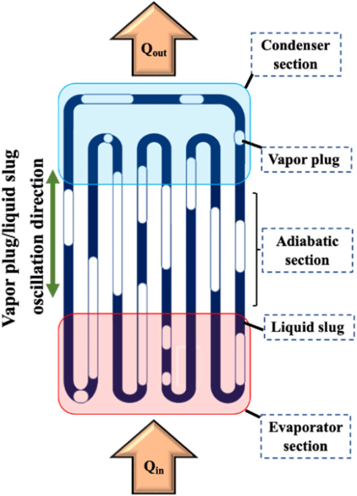
Figure 1. A schematic of an OHP
2. Oscillating heat pipe modeling
Since their invention in the 1990s by Akachi (1990, 1993), a sizable body of work concerning physical modeling of OHP function has been developed (Nikolayev, 2021). Despite much progress, these models are still insuffcient to, for example, suggest design parameters to target predefined performance metrics. The main diffculty in the development of accurate models is that the function of OHPs arises from the delicate interplay of a multitude of multiphysics phenomena taking place at various time and spatial scales. In the face of these diffculties, there has been increasing interest in machine learning methods for prediction and design (see Núñez et al., 2024). While interesting results have been obtained, the extent to which these data-driven models can accurately extrapolate to new situations is a source of concern. In fact, already in 2002, Khandekar et al. (2002) warned about this problem. In Khandekar et al. (2002), a machine learning model is trained to predict the thermal performance of a given OHP given certain operational parameters. The crucial finding of this paper is that the accuracy of these predictions deteriorated when the OHP shifted to operational regimes that were not suffciently represented in the training set. However, it should be noted that most data-driven models of OHPs do not leverage the wealth of partial, yet essential, physical knowledge developed in the field. Hybrid models resulting from the integration of physical and data-driven models can potentially address the shortcomings of each of these modeling paradigms to push new models beyond the current state-of-the-art. Techniques for developing hybrid models, some of which have been surveyed by Karniadakis et al. (2021), constitute an active area of research in computer science, mathematics, and engineering. In this investigation, subsequent sections, we adhere to the approach presented by Reyes et al. (2021) to exemplify a method of integrating physics and data. We then explore the benefits of this integration compared to models solely driven by data.
3. An example of integration of physical and data-drive models
We will consider a physical model proposed by Ma et al. (2006) in which the ensemble of liquid slugs and vapor bubbles in an OHP is modeled as a spring-mass system where slugs and plugs play the role of masses and springs, respectively. The model hinges on the assumption that all liquid slugs can be combined into a single mass and all vapor plugs into a single spring. The resulting equation of motion is
| \[ \ddot{x}+\dfrac{c}{m}\dot{x}+\dfrac{k}{m}x=\dfrac{A}{m}\Delta T(t) \] | (1) |
where \(x\) is a coordinate describing the position of the slug, \(\Delta T(t)\) is the normalized temperature difference between the evaporator and condenser, and \(m\), \(c\), \(k\), and \(A\) are constants. It is assumed that \(\Delta T(t)=1+\cos\omega t\) (Ma et al., 2006) to obtain a simplified model from which qualitative information can be extracted (Ma et al., 2006; Núñez and Ma, 2024). However, this temperature difference produces a harmonic motion of the liquid slug that is not observed in experiments. Is it possible to refine this model by learning a more realistic function \(\Delta T(t)\) from a dataset consisting only of position readings? As in the work by Reyes et al. (2021), this situation is problematic for purely data-driven techniques, as we do not have direct data pertaining to the relation that we wish to learn. To circumvent this diffculty, we must leverage the available physical knowledge of the system embodied in Eq. (1).
A synthetic dataset is built by setting \(\Delta T(t)=1+\cos\omega t\) in Eq. (1) and integrating the equation numerically with initial condition (0,0). The resulting function \(x(t)\) returns the position of the liquid slug at a given time. Even though we will not use this fact in our analysis, we know that the function \(1+\cos\omega t\) dictates the temperature difference in the synthetic dataset. This will be useful in assessing the results we obtain.
Now, replace the unknown function \(\Delta T(t)\) in Eq. (1) by an artificial neural network \(nn_{\theta}(t)\) of a given architecture (we use two hidden layers with one and two neurons) and weights \(\theta\) to form the differential equation, i.e.,
| \[ \ddot{x}+\dfrac{c}{m}\dot{x}+\dfrac{k}{m}x=\dfrac{A}{m}nn_{\theta}(t) \] | (2) |
We can now integrate this equation numerically to get a solution \(x_{\theta}(t)\). In this example, \(x(t)\) plays the role of experimental data and \(x_{\theta}(t)\) is the approximation to this data obtained by letting \(nn_{\theta}(t)\) dictate the temperature difference between evaporator and condenser. The weights \(\theta\) can be adjusted via standard techniques in machine learning until there is satisfactory agreement between \(x_{\theta}(t)\) and \(x(t)\) or, in technical terms, until a good approximation to a minimum of the loss function, i.e.,
| \[ L(\theta)=\int_{t_0}^{t_f}\left(x_{\theta}(t)-x(t)\right)^2dt \] | (3) |
is found. Figure 2 depicts the positions \(x(t)\) contained in the synthetic dataset and the prediction given by \(x_{\theta}(t)\).
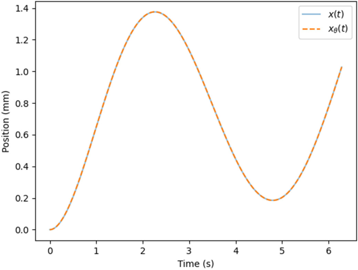
Figure 2. Comparison between the position in the synthetic dataset (solid blue) and the position predicted with the aid of the artificial neural network (dashed orange)
This agreement is not surprising as we have set up the loss function \(L(\theta)\) precisely so that \(x_{\theta}(t)\) and \(x(t)\) are very similar. More interestingly, Fig. 3 shows that the neural network \(nn_{\theta}(t)\) has also captured the temperature difference underlying the synthetic data set, even though we did not have access to readings of this variable. We have used our synthetic dataset to recover the physical model from which it arose. Furthermore, while the synthetic dataset contained data arising from a single initial condition, our trained hybrid model \(nn_{\theta}(t)\) can precisely predict the behavior of the system at any initial condition, as the differential equation itself has been recovered. In this sense, this hybrid model exhibits better extrapolation properties than it would be expected from a purely data-driven model.
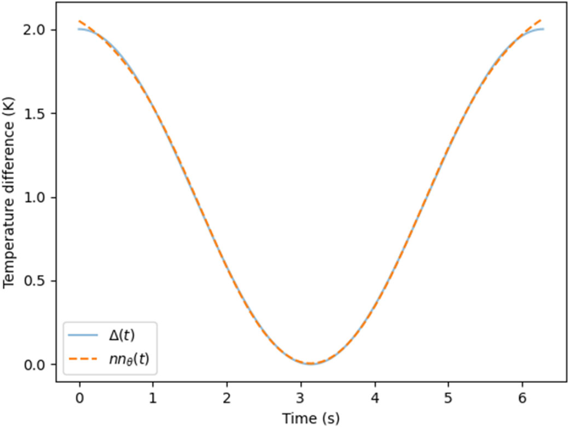
Figure 3. Comparison between the temperature difference in the synthetic dataset (solid blue) and the temperature difference predicted by the artificial neural network (dashed orange)
4. Outlook
This simple case study illustrates one technique for incorporating a data-driven component into a physical model of OHPs. One advantage of this approach is that it allows us to learn a given relation even if we do not have experimental data of that relation. At least in the case above, the hybrid model can make accurate predictions for any given initial condition, even though the synthetic data on which it was trained came from only one initial condition. Moreover, by restricting the data-driven component to a given physical relation (e.g. temperature difference), we can evaluate the physical feasibility of the trained model (e.g. is the temperature difference that we obtained reasonable?), which could indirectly lead to validating the physical model itself. However, the most suitable approach for developing a hybrid model will be dictated by both the mathematical structure of the physical model and the experimental data available. Of special interest for OHP modeling would be hybrid models aimed at capturing some of the interactions between the physics of evaporation (surface characteristic, bubble nucleation), condensation (flow regimes, wettability), and thermally excited oscillation motion, as these represent some of the most diffcult challenges for physics-based OHP modeling.
REFERENCES
Akachi, H. (1990) Structure of a Heat Pipe, US Patent No. 4,921,041.
Akachi, H. (1993) Structure of Micro-Heat Pipe, US Patent No. 5,219,020.
Karniadakis, G.E., Kevrekidis, I.G., Lu, L., Perdikaris, P., Wang, S. and Yang, L. (2021) Physics-Informed Machine Learning, Nature Reviews Physics, 3(6): 422–440.
Khandekar, S., Cui, X., and Groll, M. (2002) Thermal Performance Modeling of Pulsating Heat Pipes by Artificial Neural Network, Proceedings of 12th International Heat Pipe Conference, Moscow, Russia, June 2002.
Ma, H. (2015) Oscillating Heat Pipes, 146, New York: Springer.
Ma, H. B., Hanlon, M. A., and Chen, C. L. (2006) An Investigation of Oscillating Motions in a Miniature Pulsating Heat Pipe, Microfluids and Nanofluids, 2(2): 171–179.
Nikolayev, V.S. (2021) Physical Principles and State-of-the-Art of Modeling of the Pulsating Heat Pipe: A review, Applied Thermal Engineering, 195: 117111.
Núñez, R. and Ma, H. (2024) Transient Process Analysis of Oscillating Motion in Oscillating Heat Pipes, ASME Journal of Heat and Mass Transfer, 146(4): 043001.
Núñez, R., Mohammadian, S., Rupam, T. H., Mohammed, R., Huang, G., and Ma, H. (2024) Machine Learning for Modeling Oscillating Heat Pipes: A Review, Journal of Thermal Science and Engineering Applications, 1–20.
Reyes, B., Howard, A.A., Perdikaris, P., and Tartakovsky, A.M. (2021) Learning Unknown Physics of Non-Newtonian Fluids, Physical Review Fluids, 6(7): 073301.
References
- Akachi, H. (1990) Structure of a Heat Pipe, US Patent No. 4,921,041.
- Akachi, H. (1993) Structure of Micro-Heat Pipe, US Patent No. 5,219,020.
- Karniadakis, G.E., Kevrekidis, I.G., Lu, L., Perdikaris, P., Wang, S. and Yang, L. (2021) Physics-Informed Machine Learning, Nature Reviews Physics, 3(6): 422–440.
- Khandekar, S., Cui, X., and Groll, M. (2002) Thermal Performance Modeling of Pulsating Heat Pipes by Artificial Neural Network, Proceedings of 12th International Heat Pipe Conference, Moscow, Russia, June 2002.
- Ma, H. (2015) Oscillating Heat Pipes, 146, New York: Springer.
- Ma, H. B., Hanlon, M. A., and Chen, C. L. (2006) An Investigation of Oscillating Motions in a Miniature Pulsating Heat Pipe, Microfluids and Nanofluids, 2(2): 171–179.
- Nikolayev, V.S. (2021) Physical Principles and State-of-the-Art of Modeling of the Pulsating Heat Pipe: A review, Applied Thermal Engineering, 195: 117111.
- Núñez, R. and Ma, H. (2024) Transient Process Analysis of Oscillating Motion in Oscillating Heat Pipes, ASME Journal of Heat and Mass Transfer, 146(4): 043001.
- Núñez, R., Mohammadian, S., Rupam, T. H., Mohammed, R., Huang, G., and Ma, H. (2024) Machine Learning for Modeling Oscillating Heat Pipes: A Review, Journal of Thermal Science and Engineering Applications, 1–20.
- Reyes, B., Howard, A.A., Perdikaris, P., and Tartakovsky, A.M. (2021) Learning Unknown Physics of Non-Newtonian Fluids, Physical Review Fluids, 6(7): 073301.